The hydrology model#
This section walks through the steps in generating and updating the hydrology model which is part of the default Virtual Ecosystem configuration. The flow of key inputs, state variables, and processes are illustrated in Fig. 9.
The processes within a grid cell are loosely based on the LISFLOOD model (Van Der Knijff et al., 2010). These structure and flows of this ‘4-Bucket Model’ are summarised in Fig. 10. The processes across the model grid are loosely based on the pysheds package.

Fig. 9 Hydrology inputs, state variables, and processes in Virtual Ecosystem (click to zoom). Yellow boxes represent atmospheric input variables, green box and arrows indicate where water enters and leaves the plant model.#
Note
Calculating hydrological processes at coarse time scales is problematic and so the hydrology model uses an internal daily time step to model hydrology. When the model is run with a coarser update interval - and hence the precipitation and transpiration inputs are totals over more than one day - the hydrology model partitions the input data into daily values. Precipitation is partitioned between days assuming a gamma distribution and the total evapotranspiration is evenly divided across days.
The values returned by the hydrology model are then monthly means or monthly accumulated values.
Required variables#
The tables below show the variables that are required to initialise the hydrology model and then update it at each time step.
The model also requires several parameters that are described in detail in
HydrologyConstants.
The default values are set for forest ecosystems.
Within grid cell hydrology#
The vertical component of the hydrology model determines the water balance within each grid cell. This includes above ground processes such as rainfall, canopy interception and evaporation, leaf drainage, and surface runoff out of the grid cell. The below ground component considers infiltration, bypass flow, percolation (= vertical flow), soil moisture and soil matric potential, horizontal sub-surface runoff out of the grid cell, and changes in groundwater storage.

Fig. 10 The 4-Bucket Model represents within grid cell hydrology processes in the Virtual Ecosystem. Red solid arrows indicate upward vertical flows, red dashed arrows show vertical downward flows. The blue arrows indicate horizontal flows out of the grid cell with solid lines representing water that flows out of each layer in the current time step and dashed lines representing water that originates from upstream grid cells and flows through the grid cell directly to the stream. NOTE! Top soil and middle soil are currently treated as one layer in the model. Subsurface stormflow (Q2) and interflow (Q3) are currently not implemented; the total runoff is calculated as the sum of surface runoff (Q1) and the flows out of the groundwater buckets (=subsurface runoff, Q4+Q5).#
Rainfall generator#
To generate daily rainfall, we combine three steps: rainfall occurrence is simulated using a first-order Markov chain, rainfall intensity on wet days is drawn from a Gamma distribution, and a final scaling step is applied (Katz, 1977). Together, these components provide a simple yet realistic stochastic rainfall model.
Wet/Dry rainfall occurrence model#
A Markov chain is a stochastic (random) process in which the probability of the current state depends only on the previous state, not on the full history. This is known as the Markov property.
Let \(S_t\) be the rainfall state on day \(t\):
Because this is a first-order Markov chain, the probability of rain today depends only on whether it rained yesterday:
where:
\(p_{ww}\) is the probability that a wet day follows a wet day,
\(p_{wd}\) is the probability that a wet day follows a dry day.
This structure captures the tendency of rainfall to occur in clusters (e.g., wet spells and dry spells), which would not be reproduced by independent random sampling.
Rainfall intensity model#
On days classified as wet (\(S_t = 1\)), rainfall amounts are generated independently from a Gamma distribution:
The Gamma distribution is commonly used for rainfall because:
it only produces positive values,
it can represent skewed distributions (many small events, few large ones),
its shape can be adjusted using parameters.
where:
\(k\) is the shape parameter (controls variability),
\(\theta\) is the scale parameter (controls magnitude).
Monthly scaling#
The sampled daily intensities \(x_i\) are relative values and do not yet match a target monthly rainfall total. To ensure consistency with observed or prescribed totals, they are rescaled:
where:
\(r_i\) is the rainfall on day \(i\) [mm],
\(x_i\) is the sampled Gamma intensity,
\(P\) is the total monthly rainfall [mm],
\(n\) is the number of wet days in the month.
This scaling preserves the relative distribution of rainfall across wet days while ensuring that the total rainfall equals the desired monthly value.
Canopy interception#
Canopy interception is estimated using the following storage-based equation after Aston (1979) and Merriam (1960) as implemented in Van Der Knijff et al. (2010):
where \(Int\) (mm) is the interception per time step, \(S_{max}\) (mm) is the maximum interception, \(R\) (mm) is the rainfall intensity per time step and the factor \(k\) accounts for the density of the vegetation.
\(S_{max}\) is calculated using an empirical equation (Von Hoyningen-Huene, 1981):
where LAI is the average Leaf Area Index (m2 m-2). \(k\) is estimated as:
Canopy evaporation and leaf drainage#
Evaporation of intercepted water from the canopy following the LISFLOOD model Van Der Knijff et al. (2010). The maximum evaporation per time step \(EW_{max}\) is proportional to the fraction of vegetated area:
where \(EW_{0}\) is the potential evaporation rate, the dimensionless constant \(\kappa_{gb}\) is the extinction coefficient for global solar radiation. In LISFLOOD, \(\kappa_{gb}\) is given by the product \(0.75 \cdot \kappa_{df}\), where \(\kappa_{df}\) is the extinction coefficient for diffuse visible light: its value is provided as input to the model and it varies between 0.4 and 1.1.
The actual amount of evaporation \(EW_{int}\) is limited by the amount of water stored on the leaves \(Int_{cum}\):
Another amount of water falls to the soil because of leaf drainage which is typically modelled as a linear reservoir:
where \(D_{int}\) is the amount of leaf drainage per time step and \(T_{int}\) is a time constant (or residence time) of the interception store. Setting \(T_{int} = 1\) day is strongly recommended and means that all the water in the interception store evaporates or falls to the soil surface as leaf drainage within one day. Given the daily timestep of the model, this means that we don’t account for this step explicitly.
Water at the surface#
Precipitation that reaches the surface is defined as incoming precipitation minus canopy evaporation (plus leaf drainage if modelled explicitly) plus condensation (calculated in abiotic model). The water at the surface can follow different trajectories: runoff at the surface, remain at the surface as searchable resource for animals, return to the atmosphere via evaporation, or infiltrate into the soil where it can be taken up by plants or percolate to the groundwater.
Surface Runoff#
Surface runoff is calculated with a simple bucket model based on Davis et al. (2017): if precipitation exceeds top soil moisture capacity , the excess water is added to runoff and top soil moisture is set to soil moisture capacity value; if the top soil is not saturated, precipitation is added to the current soil moisture level and runoff is set to zero.
Searchable resource#
Some of the water that lands on the surface is stored in depressions as puddles or larger standing water that is a searchable resources for animals. This is currently not implemented.
Evaporation#
The implementation of soil evaporation is based on classical bulk aerodynamic formulation. We use the so-called ‘alpha’ method to estimate the evaporative flux (Mahfouf and Noilhan, 1991) and the implementation by Barton (1979):
where \(\Theta\) is the available top soil moisture (here relative soil moisture) , \(E_{g}\) is the evaporation flux (W m-2), \(\rho_{air}\) is the density of air (kg m-3), \(R_{a}\) is the aerodynamic resistance (unitless), \(q_{sat}(T_{s})\) (unitless) is the saturated specific humidity, and \(q_{g}\) is the specific soil moisture near the surface (unitless).
In a final step, the bare soil evaporation is adjusted to shaded soil evaporation Supit et al. (1994):
where \(\kappa_{gb}\) is the extinction coefficient for global radiation, and \(LAI\) is the total leaf area index.
Infiltration#
Infiltration is currently handled in a very simplistic way: the water that ‘fits in the topsoil bucket’ is added to the topsoil layer. We aim to implement a more realistic process that accounts for soil type specific infiltration capacities.
Bypass flow#
Bypass flow is here defined as the flow that bypasses the soil matrix and drains directly to the groundwater. During each time step, a fraction of the water that is available for infiltration is added to the groundwater directly (i.e. without first entering the soil matrix). It is assumed that this fraction is a power function of the relative saturation of the superficial and upper soil layers. This results in the following equation (after Van Der Knijff et al. (2010)):
\(D_{pref, gw}\) is the amount of preferential flow per time step (mm), \(W_{av}\) is the amount of water that is available for infiltration, and \(c_{pref}\) is an empirical shape parameter. This parameter affects how much of the water available for infiltration goes directly to groundwater via preferential bypass flow; a value of 0 means all surface water goes directly to groundwater, a value of 1 gives a linear relation between soil moisture and bypass flow. The equation returns a preferential flow component that becomes increasingly important as the soil gets wetter.
Vertical flow#
To calculate the flow of water through unsaturated soil, we combine Richards’ equation and Darcy’s law for unsaturated flow. First, we calculate the effective saturation \(S_{e}\) and effective unsaturated hydraulic conductivity \(K(\Theta)\) based on the moisture content \(\Theta\) using the van Genuchten - Mualem model (Van Genuchten (1980), Mualem (1976)).
First, the effective saturation is calculated as:
where \(\Theta_{r}\) is the soil moisture residual and \(\Theta_{s}\) is the soil moisture saturation.
Then, the effective unsaturated hydraulic conductivity is computed as:
where \(K_{s}\) is the saturated hydraulic conductivity, \(L\) is the pore connectivity parameter (assumed to be 0.5 in most of studies), and \(m=1-1/n\) is a shape parameter derived from the non-linearity parameter \(n\).
The soil matric potential \(\Psi_{m}\) is calculated as follows:
where \(\alpha\) is the inverse of air entry value.
Then, the function applies Darcy’s law to calculate the water flow rate \(q\) in \(\frac{mm}{day^1}\) considering the effective unsaturated hydraulic conductivity:
where \(\frac{d \Psi_{m}}{dz}\) is the soil matric potential gradient with \(z\) the elevation (gravitational potential) or gravitational head.
Note
There are severe limitations to this approach on the temporal and spatial scale of this model and this can only be treated as a very rough approximation!
Soil moisture redistribution#
Soil moisture is updated for each layer by removing the vertical flow of the current layer and adding it to the layer below. The implementation is based on Van Der Knijff et al. (2010). Additionally, the canopy transpiration is removed from the second soil layer.
Note
We do currently NOT include any horizontal flows from the soil layers towards the stream (Q2 and Q3 in Fig. 10).
Belowground runoff and groundwater storage#
Groundwater storage and runoff towards the channel are modelled using two parallel linear reservoirs, similar to the approach used in the HBV-96 model (Lindström et al., 1997) and the LISFLOOD (Van Der Knijff et al., 2010) (see for full documentation).
The upper zone represents a quick runoff component, which includes fast groundwater and (vertical) subsurface flow through macro-pores in the soil. The lower zone represents the slow groundwater component that generates the base flow.
The runoff from the upper zone to the channel, \(Q_{uz}\), (mm), (Q4 in Fig. 10) equals:
where \(T_{uz}\) is the reservoir constant for the upper groundwater layer (days), and \(UZ\) is the amount of water that is stored in the upper zone (mm). The amount of water stored in the upper zone is computed as follows:
where \(D_{ls,gw}\) is the flow from the lower soil layer to groundwater, \(D_{pref,gw}\) is the amount of preferential flow or bypass flow per time step, \(D_{uz,lz}\) is the amount of water that percolates from the upper to the lower zone, all in (mm).
The water percolates from the upper to the lower zone is the inflow to the lower groundwater zone. This amount of water is provided by the upper groundwater zone. \(D_{uz,lz}\) is a fixed amount per computational time step and it is defined as follows:
where \(GW_{perc}\), [mm day-1], is the maximum percolation rate from the upper to the lower groundwater zone. The runoff from the lower zone to the channel \(Q_{lz}\), (mm), (Q5 in Fig. 10) is then computed by:
\(T_{lz}\) is the reservoir constant for the lower groundwater layer, (days), and \(LZ\) is the amount of water that is stored in the lower zone, (mm). \(LZ\) is computed as follows:
where \(D_{uz,lz}\) is the percolation from the upper groundwater zone, (mm), and \(GW_{loss}\) is the maximum percolation rate from the lower groundwater zone, (mm day-1).
The amount of water defined by \(GW_{loss}\) never rejoins the river channel and is lost beyond the catchment boundaries or to deep groundwater systems. The larger the value of \(GW_{loss}\), the larger the amount of water that leaves the system.
Across grid hydrology#
The second part of the hydrology model calculates the horizontal water movement across the full model grid including surface runoff and sub-surface runoff, combined into local runoff generation per grid cell and total runoff across the grid.
Hereinafter, we refer to river discharge rate to indicate the amount of water passing a particular point of a river (m3 s−1), whereas runoff \(R\) is regarded as the depth of water produced from a drainage area during a particular time interval (mm).
Drainage map#
The flow direction of water above and below ground is based on a digital elevation model which needs to be provided as a NetCDF file at the start of the simulation. Here is a description of the steps that happen during the hydrology model initialisation (plotting only for illustration):
# Read elevation data from NetCDF
import numpy as np
import xarray as xr
from xarray import DataArray

input_file = "../../_static/river_DEM.nc"
digital_elevation_model = xr.open_dataset(input_file)
elevation = digital_elevation_model["elevation"]
# Create Grid and Data objects and add elevation data
from virtual_ecosystem.core.grid import Grid
from virtual_ecosystem.core.data import Data

grid = Grid(
    grid_type="square", cell_area=8100, cell_nx=9, cell_ny=9, xoff=-45, yoff=-45
)
data = Data(grid=grid)
data["elevation"] = elevation

# Plot elevation data on grid
import matplotlib.pyplot as plt
from matplotlib import colors

ele_plot = DataArray(
    data["elevation"].to_numpy().reshape((9, 9)),
    dims=("x", "y"),
    coords={"x": np.arange(9), "y": np.arange(9)},
)
plt.figure(figsize=(10, 6))
ele_plot.plot(cmap="terrain")
plt.title("Elevation, [m]")
plt.xlabel("x")
plt.ylabel("y")
plt.show()
[INFO] - data - __setitem__(235) - Adding data array for 'elevation'
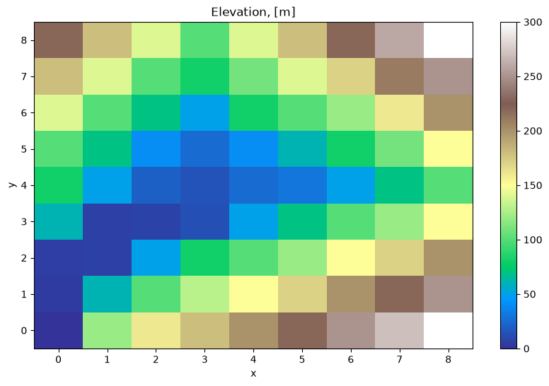
The initialisation step of the hydrology model finds all the neighbours for each grid
cell and determine which neighbour has the lowest elevation. The code below returns the
neighbours of the grid cell with cell_id = 56 as an example.
grid.set_neighbours(distance=100)
grid.neighbours[56]
array([47, 55, 56, 57, 65])
Based on that relationship, the model determines all upstream neighbours
for each grid cell and creates a drainage map, i.e. a dictionary that contains for each
grid cell all upstream grid cells. For example, cell_id = 34 has upstream cells
with the indices [4, 13, 22]. This gives the flow direction.
from virtual_ecosystem.models.hydrology.above_ground import calculate_drainage_map

drainage_map = calculate_drainage_map(
    grid=grid,
    elevation=np.array(data["elevation"]),
)
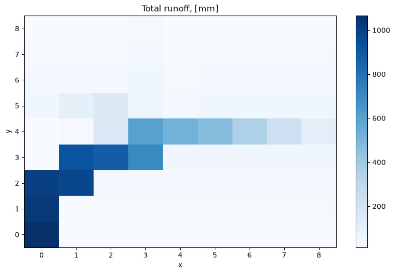
Runoff and river discharge rate#
We track horizontal water fluxes in two pathways — surface and subsurface runoff — and then combine them into total runoff, which can be converted to river discharge rate.
Surface runoff (\(R_{surface}\))#
Water moving over the land surface into the river channel. For each cell, this includes:
Local surface runoff: water generated within the cell during the current timestep.
Upstream surface runoff: surface runoff generated in all upstream cells during the same timestep.
Subsurface runoff (\(R_{subsurface}\))#
Water moving laterally through soil and groundwater pathways towards the river channel. For each cell, this includes:
Local subsurface runoff: lateral + baseflow generated in the cell during the current timestep.
Upstream subsurface runoff: subsurface runoff generated in upstream cells during the same timestep.
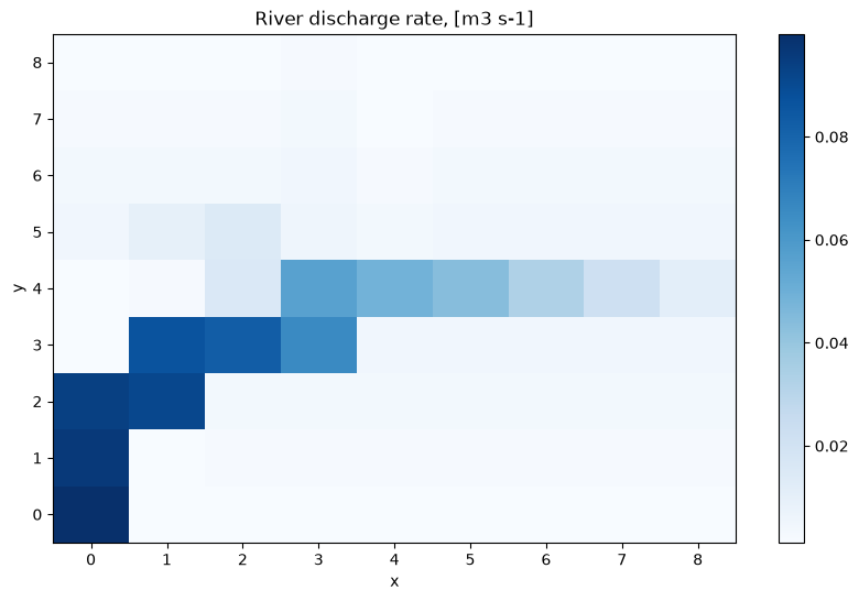
Total runoff (\(R_{total}\)) and river discharge rate#
The total water volume passing through a cell is the sum of these two pathways:
This total volume can then be converted to a river discharge rate in cubic meters per second (m3 s-1) using cell area and unit conversions.
from virtual_ecosystem.models.hydrology.above_ground import route_horizontal_flow

# Local runoff
subsurface_runoff = DataArray(np.full_like(data["elevation"], 1.0), dims="cell_id")
surface_runoff = DataArray(np.full_like(data["elevation"], 12), dims="cell_id")

# Total runoff = local runoff generation + upstream inflow
total_runoff = route_horizontal_flow(
    drainage_map=drainage_map,
    surface_runoff=surface_runoff,
    subsurface_runoff=subsurface_runoff,
)

# Reshape to 9x9 grid and plot total runoff map
reshaped_runoff = DataArray(
    total_runoff.reshape((9, 9)),
    dims=("x", "y"),
    coords={"x": np.arange(9), "y": np.arange(9)},
)

plt.figure(figsize=(10, 6))
reshaped_runoff.plot(cmap="Blues")
plt.title("Total runoff, [mm]")
plt.xlabel("x")
plt.ylabel("y")
plt.show()
from virtual_ecosystem.models.hydrology.above_ground import (
    convert_mm_flow_to_m3_per_second,
)

# Convert total runoff [mm] to river discharge rate [m3 s-1]
river_discharge_rate = convert_mm_flow_to_m3_per_second(
    river_discharge_mm=total_runoff,
    area=grid.cell_area,
    days=1,
    seconds_to_day=86400,
    meters_to_millimeters=1000,
)

# Reshape to 9x9 grid and plot river discharge rate
reshaped_discharge_rate = DataArray(
    river_discharge_rate.reshape((9, 9)),
    dims=("x", "y"),
    coords={"x": np.arange(9), "y": np.arange(9)},
)

plt.figure(figsize=(10, 6))
reshaped_discharge_rate.plot(cmap="Blues")
plt.title("River discharge rate, [m3 s-1]")
plt.xlabel("x")
plt.ylabel("y")
plt.show()
Note
To close the water balance, water needs to enter and leave the grid at some point. These boundaries are currently not implemented.
Generated variables#
The calculations described above result in the following variables being calculated and saved within the data object, and then updated
Updated variables#
The link below provides the complete set of model variables that are updated at each model step.