Using the Virtual Ecosystem#

This page provides a brief demonstration of the Virtual Ecosystem model in operation. Once you have installed the Virtual Ecosystem, you should be able to replicate this example on your own computer using the commands below.

Example model data#

The demonstration requires an installation of the example data provided with the Virtual Ecosystem package. If you have previously attempted to run this example then the simulation will refuse to overwrite existing output files. You can either:

delete the existing example data folder and reinstall it,
create a fresh installation using a different location, or
create and use a new output directory with the existing example data folder.

It is worth re-reading the example data page to get an overview of the directory structure and the configuration and data files.

The `ve_run` command#

You’ve already used this command to install the example data but most of the options to the ve_run command are used to run the simulation. The --help option can be used to show the various arguments that can be used to set how a model runs:

macOS/Linux

ve_run --help

Windows (CMD)

ve_run --help

Windows (Powershell)

ve_run --help

usage: ve_run [-h] [--version] [--install-example INSTALL_EXAMPLE]
              [-o OUTPATH] [-c CLI_CONFIG] [--logfile LOGFILE] [-q]
              [cfg_paths ...]

Configure and run a Virtual Ecosystem simulation.

This program sets up and runs a Virtual Ecosystem simulation. The program expects
to be provided with paths to TOML formatted configuration files for the simulation.
The configuration is modular: a directory path can be used to add all TOML
configuration files in the directory, or individual file paths can be used to select
specific combinations of configuration files. These are combined and validated and
then used to initialise and run the model.

As an alternative to providing configuration paths, the `--install-example` option
allows users to provide a location where a simple example set of datasets and
configuration files provided with the Virtual Ecosystem package can be installed.
This option will create a `ve_example` directory in the location, and users can
examine the input files and run the simulation from that directory:

`ve_run /provided/install/path/ve_example`

The output directory for simulation results is typically set in the configuration
files, but can be overwritten using the `--outpath` option. A log file path can be
provided for logging output. If this is not provided then the log will be written to
the console, but the logging is typically verbose and it is usually better to
redirect the log to a file.

When logging is redirected to a file, a short progress report is written to stdout.
By default, the command reports: the start and end of the simulation and log
location; the completion of simulation stages; and a progress bar over the time
steps of the model. The `--quiet` command can be used to incrementally mute this
output: `-q` will remove the progress bar, `-qq` just prints the start and stop and
`-qqq` mutes the report entirely.

The `--config` option can be used to override configuration settings provided in the
file or to add additional settings. This is typically used to run a set of parallel
simulations that vary configuration settings of interest around a central
configuration setup, without the need to write a specific configuration file for
each permutation.

The resolved complete configuration will then be written to a single consolidated
config file in the output path with a default name of
`ve_full_model_configuration.toml`. This can be disabled by setting the
`core.data_output_options.save_merged_config` option to false. Note that the merged
configuration automatically converts all file paths within the merged configurations
to absolute file paths - this ties the merged configuration to the file system where
the run is executed.

positional arguments:
  cfg_paths             Paths to config files

options:
  -h, --help            show this help message and exit
  --version             show program's version number and exit
  --install-example INSTALL_EXAMPLE
                        Install the Virtual Ecosystem example data to the
                        given location
  -o, --outpath OUTPATH
                        Path for output files
  -c, --config CLI_CONFIG
                        Override configuration settings
  --logfile LOGFILE     A file path to use for logging a Virtual Ecosystem
                        simulation
  -q, --quiet           Quieten the default progress reporting

Running the example model#

The code below runs a simulation using the example data. The command uses the command line options to set three things:

It points to the files in config directory that should be used configure the model. N.B. this directory contains configuration for all possible model combinations so providing just the config directory as a path will result in an invalid configuration.
It sets the output directory to be used by the simulation to out. You could create a new output directory (e.g. out_test_2) and change this to run a new simulation using the existing data.
It redirects the model logging to a file in the output directory, rather than printing it all to screen.

When the detailed logging is redirected to a file, the command generates a short progress report to show the model running. This can be made shorter or completely muted by using the -q argument: repeat the argument to remove more details (e.g. -qq or -qqq).

Warning

If the path provided for the log points to a file that already exists the detailed logging is added to the end of the file rather than creating a new file. We would recommend creating a new logfile for each simulation as reusing files in this way can create confusion.

In the example code below, the ve_example folder has been previously installed under the directory /tmp/

macOS/Linux

ve_run /tmp/ve_example/config/data_config.toml \
    /tmp/ve_example/config/abotic_config.toml \
    /tmp/ve_example/config/animal_config.toml \
    /tmp/ve_example/config/hydrology_config.toml \
    /tmp/ve_example/config/litter_config.toml \
    /tmp/ve_example/config/plant_config.toml \
    /tmp/ve_example/config/soil_config.toml \
    --out /tmp/ve_example/out \
    --logfile /tmp/ve_example/out/logfile.log

Windows (CMD)

ve_run C:\tmp\ve_example\config\data_config.toml ^
    C:\tmp\ve_example\config\abotic_config.toml ^
    C:\tmp\ve_example\config\animal_config.toml ^
    C:\tmp\ve_example\config\hydrology_config.toml ^
    C:\tmp\ve_example\config\litter_config.toml ^
    C:\tmp\ve_example\config\plant_config.toml ^
    C:\tmp\ve_example\config\soil_config.toml ^
    --out C:\tmp\ve_example\out ^
    --logfile C:\tmp\ve_example\logfile.log

Windows (Powershell)

ve_run C:\tmp\ve_example\config\data_config.toml `
    C:\tmp\ve_example\config\abotic_config.toml `
    C:\tmp\ve_example\config\animal_config.toml `
    C:\tmp\ve_example\config\hydrology_config.toml `
    C:\tmp\ve_example\config\litter_config.toml `
    C:\tmp\ve_example\config\plant_config.toml `
    C:\tmp\ve_example\config\soil_config.toml `
    --out C:\tmp\ve_example\out `
    --logfile C:\tmp\ve_example\logfile.log

Starting Virtual Ecosystem simulation.
Logging to: ve_example/out/logfile.log
* Loading configuration
* Saved compiled configuration: ve_example/out/ve_full_model_configuration.toml
* Built core model components
* Initial data loaded
* Models initialised: soil, hydrology, abiotic, animal, litter, plants
* Saved model initial state
* Starting simulation
100%|██████████| 24/24 [00:50<00:00,  2.12s/it]
* Simulation completed
* Merged time series data
* Saved final model state
Virtual Ecosystem run complete.

The log file is very long and shows the step by step process of running the model - it is primarily used for diagnosing problems with the model. You can view a sample of the contents in the dropdown below:

Partial log output

[INFO] - config_builder - _collect_config_paths(416) - Config paths resolve to 5 files
[INFO] - config_builder - _load_config_toml(439) - Config TOML loaded from ve_example/config/soil_microbial_groups.toml
[INFO] - config_builder - _load_config_toml(439) - Config TOML loaded from ve_example/config/ve_run.toml
[INFO] - config_builder - _load_config_toml(439) - Config TOML loaded from ve_example/config/plant_config.toml
[INFO] - config_builder - _load_config_toml(439) - Config TOML loaded from ve_example/config/data_config.toml
[INFO] - config_builder - _load_config_toml(439) - Config TOML loaded from ve_example/config/animal_config.toml
[INFO] - config_builder - _compile_data(363) - Configuration data compiled.
[INFO] - registry - register_module(91) - Registering module: virtual_ecosystem.models.soil
[INFO] - registry - get_model(161) - Registering model class for virtual_ecosystem.models.soil: SoilModel
[INFO] - registry - register_module(104) - Configuration class registered for virtual_ecosystem.models.soil
[INFO] - registry - register_module(91) - Registering module: virtual_ecosystem.core
[INFO] - registry - register_module(104) - Configuration class registered for virtual_ecosystem.core
[INFO] - registry - register_module(91) - Registering module: virtual_ecosystem.models.hydrology
[INFO] - registry - get_model(161) - Registering model class for virtual_ecosystem.models.hydrology: HydrologyModel
[INFO] - registry - register_module(104) - Configuration class registered for virtual_ecosystem.models.hydrology
[INFO] - registry - register_module(91) - Registering module: virtual_ecosystem.models.abiotic
[INFO] - registry - get_model(161) - Registering model class for virtual_ecosystem.models.abiotic: AbioticModel
[INFO] - registry - register_module(104) - Configuration class registered for virtual_ecosystem.models.abiotic
[INFO] - registry - register_module(91) - Registering module: virtual_ecosystem.models.animal
[INFO] - registry - get_model(161) - Registering model class for virtual_ecosystem.models.animal: AnimalModel
--- many lines omitted ---
[INFO] - data - __setitem__(233) - Replacing data array for 'soil_n_pool_necromass'
[INFO] - data - __setitem__(233) - Replacing data array for 'soil_n_pool_maom'
[INFO] - data - __setitem__(233) - Replacing data array for 'soil_n_pool_ammonium'
[INFO] - data - __setitem__(233) - Replacing data array for 'soil_n_pool_nitrate'
[INFO] - data - __setitem__(233) - Replacing data array for 'soil_p_pool_dop'
[INFO] - data - __setitem__(233) - Replacing data array for 'soil_p_pool_particulate'
[INFO] - data - __setitem__(233) - Replacing data array for 'soil_p_pool_necromass'
[INFO] - data - __setitem__(233) - Replacing data array for 'soil_p_pool_maom'
[INFO] - data - __setitem__(233) - Replacing data array for 'soil_p_pool_primary'
[INFO] - data - __setitem__(233) - Replacing data array for 'soil_p_pool_secondary'
[INFO] - data - __setitem__(233) - Replacing data array for 'soil_p_pool_labile'
[INFO] - data - __setitem__(233) - Replacing data array for 'production_of_fungal_fruiting_bodies'
[INFO] - data - __setitem__(233) - Replacing data array for 'dissolved_nitrate'
[INFO] - data - __setitem__(233) - Replacing data array for 'dissolved_ammonium'
[INFO] - data - __setitem__(233) - Replacing data array for 'dissolved_phosphorus'
[INFO] - data - __setitem__(233) - Replacing data array for 'ecto_supply_limit_n'
[INFO] - data - __setitem__(233) - Replacing data array for 'ecto_supply_limit_p'
[INFO] - data - __setitem__(233) - Replacing data array for 'arbuscular_supply_limit_n'
[INFO] - data - __setitem__(233) - Replacing data array for 'arbuscular_supply_limit_p'
[INFO] - main - ve_run(308) - Virtual Ecosystem model run completed!

Looking at the results#

The Virtual Ecosystem writes out a number of data files:

initial_state.nc: A single compiled file of the initial input data.
all_continuous_data.nc: An optional record of time series data of the variables updated at each time step.
final_state.nc: The model data state at the end of the final step.

These files are written to the standard NetCDF data file format: below, we use the xarray and matplotlib Python packages to load and visualise this data. You may need to install these to replicate these outputs on your own computer.

import matplotlib.pyplot as plt
import numpy as np
import xarray

# Load the generated data files
initial_state = xarray.load_dataset("ve_example/out/initial_state.nc")
continuous_data = xarray.load_dataset("ve_example/out/all_continuous_data.nc")
final_state = xarray.load_dataset("ve_example/out/final_state.nc")

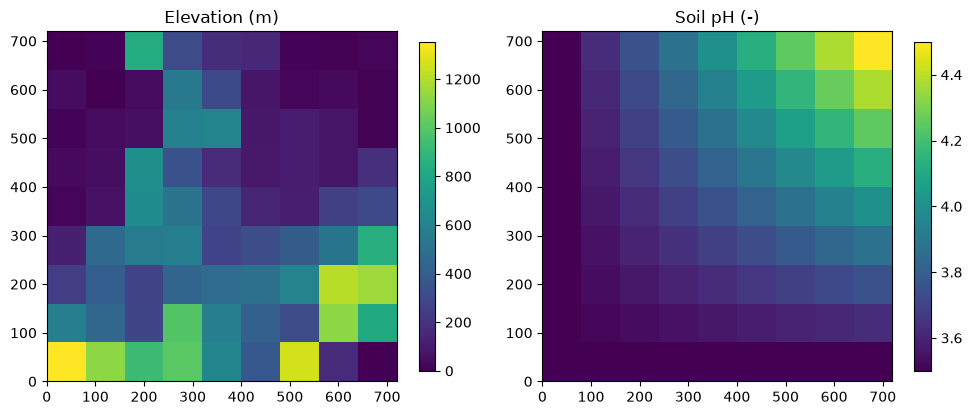
Initial state and input data#

The initial_state.nc file contains all of the data required to run the model. For some variables - such as elevation and soil pH - this just provides the constant value for each grid cell than will then be used throughout the simulation. For other variables - such as the litter pool sizes - the values provided are initial values which wil be updated as the simulation runs. Finally, for some variables - such as precipitation and temperature - a time series is provided which is used to that drive (or force) the behaviour of the model through time.

extent = [
    float(initial_state.x.min()),
    float(initial_state.x.max()),
    float(initial_state.y.min()),
    float(initial_state.y.max()),
]

# Make two side by side plots
fig, (ax1, ax2) = plt.subplots(ncols=2, figsize=(10, 5))

# Elevation
im1 = ax1.imshow(initial_state["elevation"].to_numpy().reshape((9, 9)), extent=extent)
ax1.set_title("Elevation (m)")
fig.colorbar(im1, ax=ax1, shrink=0.7)

# Initial soil carbon
im2 = ax2.imshow(initial_state["pH"].to_numpy().reshape((9, 9)), extent=extent)
ax2.set_title("Soil pH (-)")
fig.colorbar(im2, ax=ax2, shrink=0.7)

plt.tight_layout()

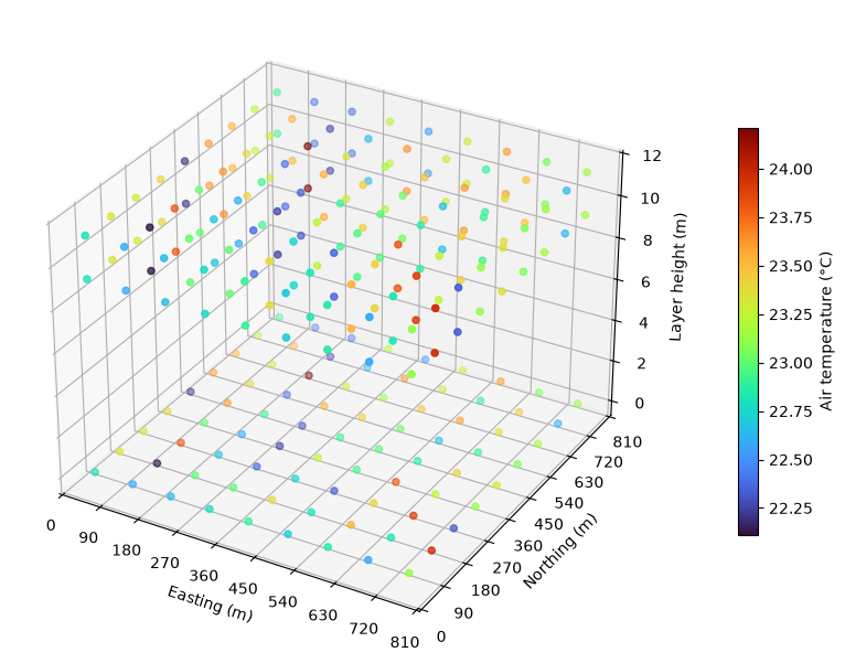
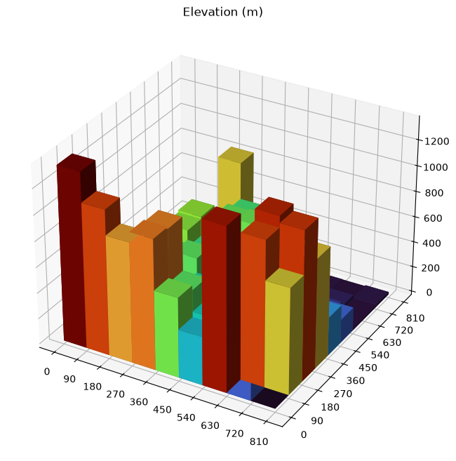
../_images/365b327978624496214f5d01eebe5b0f90cedd889092748a1ed4d06b0bd3093f.png

For some variables, it may be useful to visualise spatial structure in 3 dimensions. The obvious candidate is elevation.

# Extract the elevation data for a 3D plot
top = initial_state["elevation"].to_numpy()
x = continuous_data["x"].to_numpy()
y = continuous_data["y"].to_numpy()
bottom = np.zeros_like(top)
width = depth = 90

# Make a 3D barplot of the elevation
fig = plt.figure(figsize=(10, 8))
ax = fig.add_subplot(projection="3d")
colors = plt.cm.turbo(top.flatten() / float(top.max()))

poly = ax.bar3d(x, y, bottom, width, depth, top, shade=True, color=colors)
ax.set_title("Elevation (m)")

cell_bounds = range(0, 811, 90)
ax.set_xticks(cell_bounds)
_ = ax.set_yticks(cell_bounds)

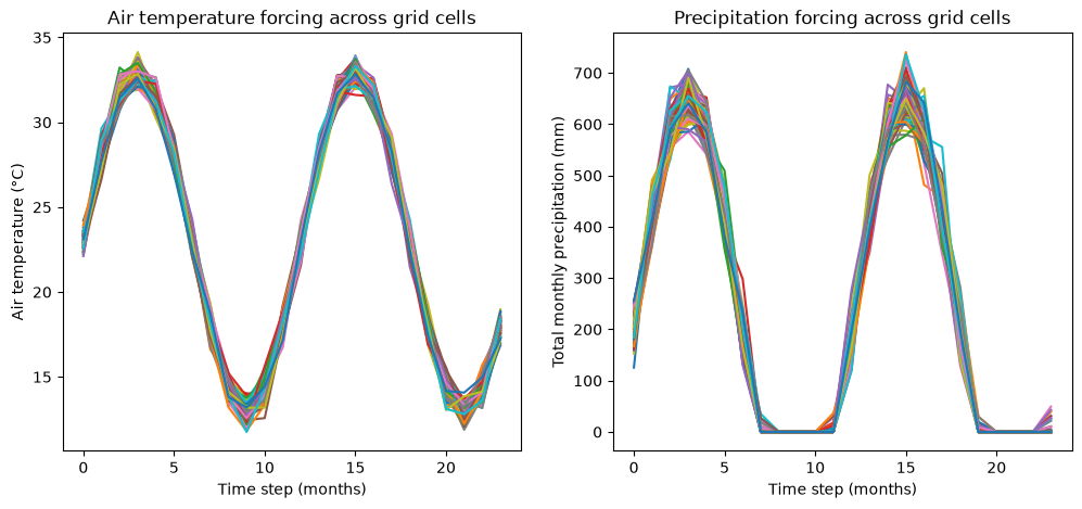
../_images/930bf097e528b70ce9472cf37b6709662910cd662128223a8bf6afb65565e556.png

For other variables, such as air temperature and precipitation, the initial data also provides time series data at reference height that are used to force the simulation across the configured time period.

initial_state

<xarray.Dataset> Size: 453kB
Dimensions:                               (cell_id: 81, time_index: 24, pft: 2,
                                           element: 3, layers: 14,
                                           community_id: 81,
                                           functional_group_id: 15,
                                           groundwater_layers: 2, dim_0: 81)
Coordinates:
  * cell_id                               (cell_id) int64 648B 0 1 2 ... 79 80
  * time_index                            (time_index) int64 192B 0 1 ... 22 23
  * pft                                   (pft) <U9 72B 'broadleaf' 'shrub'
  * element                               (element) <U1 12B 'C' 'N' 'P'
  * layers                                (layers) int64 112B 0 1 2 ... 11 12 13
  * community_id                          (community_id) int64 648B 0 1 ... 80
  * functional_group_id                   (functional_group_id) <U20 1kB 'car...
    x                                     (cell_id) int32 324B 0 90 ... 630 720
    y                                     (cell_id) int32 324B 720 720 ... 0 0
    layer_roles                           (layers) <U7 392B 'above' ... 'subs...
Dimensions without coordinates: groundwater_layers, dim_0
Data variables: (12/105)
    air_temperature_ref                   (cell_id, time_index) float64 16kB ...
    relative_humidity_ref                 (cell_id, time_index) float64 16kB ...
    atmospheric_pressure_ref              (cell_id, time_index) float64 16kB ...
    precipitation                         (cell_id, time_index) float64 16kB ...
    atmospheric_co2_ref                   (cell_id, time_index) float64 16kB ...
    mean_annual_temperature               (cell_id) float64 648B 23.0 ... 23.0
    ...                                    ...
    ecto_supply_limit_n                   (dim_0) float64 648B 0.0 0.0 ... 0.0
    ecto_supply_limit_p                   (dim_0) float64 648B 0.0 0.0 ... 0.0
    arbuscular_supply_limit_n             (dim_0) float64 648B 0.0 0.0 ... 0.0
    arbuscular_supply_limit_p             (dim_0) float64 648B 0.0 0.0 ... 0.0
    production_of_fungal_fruiting_bodies  (cell_id) float64 648B 0.0 0.0 ... 0.0
    timestamp                             (time_index) datetime64[ns] 192B 20...

xarray.Dataset

Dimensions:
- cell_id: 81
- time_index: 24
- pft: 2
- element: 3
- layers: 14
- community_id: 81
- functional_group_id: 15
- groundwater_layers: 2
- dim_0: 81

Coordinates: (10)

Data variables: (105)

# Make two side by side plots
fig, (ax1, ax2) = plt.subplots(ncols=2, figsize=(12, 5))

# Air temperature
ax1.plot(initial_state["time_index"], initial_state["air_temperature_ref"].T)
ax1.set_title("Air temperature forcing across grid cells")
ax1.set_ylabel("Air temperature (°C)")
ax1.set_xlabel("Time step (months)")

# Precipitation
ax2.plot(initial_state["time_index"], initial_state["precipitation"].T)
ax2.set_title("Precipitation forcing across grid cells")
ax2.set_ylabel("Total monthly precipitation (mm)")
_ = ax2.set_xlabel("Time step (months)")

../_images/70b69e8dc1baacf7bacaaa8d05abfcab8fbd2656a3e6e36aaf06a4df4ae77849.png

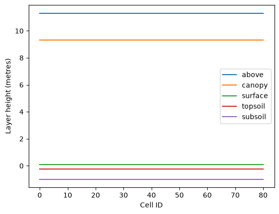
Model outputs#

The main output of interest is the all_continuous_data.nc file, which contains variables describing the change in the models through the simulation process. To keep the size of this file down only variables updated by a model are included, which means things like soil pH and input climatic data are not included. It also only contains the values of variables after they have been updated, so the time series runs from the first to final time step, i.e. the initial value of each variable is excluded. As the data contained in this file has a time dimension, we can visualise it across time. This can happen in a number of formats such as spatial grids, individual time series within grid cells and as the three dimensional structure of the vertical layers within the simulation. We describe these plotting processes below.

If you only want to compare the initial and final states of the model, you instead would want to use the final_state.nc file which provides the full final state of the model, i.e. is effectively the equivalent of initial_state.nc for the final time step (see above for plotting suggestions).

Warning

At present when the Virtual Ecosystem reads in netCDF data it flips it (i.e. the spatial x dimension becomes the y dimension and vice versa). This doesn’t affect the simlation, but does need to be corrected for when analysing the spatial outputs, which will be flipped.

Spatial data#

Using the soil carbon held as mineral-associated organic matter as an example:

# Make three side by side plots
fig, axes = plt.subplots(ncols=3, figsize=(10, 5))

# Plot start and end MAOM
val_min = continuous_data["soil_c_pool_maom"].min()
val_max = continuous_data["soil_c_pool_maom"].max()

# Plot 3 time slices
for idx, ax in zip([0, 10, 23], axes):
    im = ax.imshow(
        continuous_data["soil_c_pool_maom"][idx, :].to_numpy().reshape((9, 9)),
        extent=extent,
        vmax=val_max,
        vmin=val_min,
    )
    ax.set_title(f"Time step: {idx}")

fig.colorbar(im, ax=axes, orientation="vertical", shrink=0.5)
_ = plt.suptitle("Soil carbon: mineral-associated organic matter", y=0.78, x=0.45)

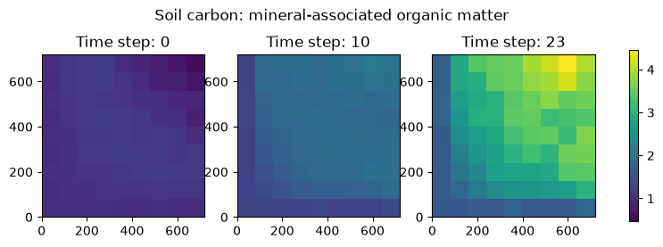
../_images/ad7d31180549d0231070c4ea1cba0c855dff305b1a373d32e02086be4644f355.png

Temporal data#

The plot below shows the mineral-associated organic matter data as a time series showing the values in each cell across time.

plt.plot(continuous_data["time_index"], continuous_data["soil_c_pool_maom"])
plt.xlabel("Time step")
_ = plt.ylabel("Soil carbon as MAOM")

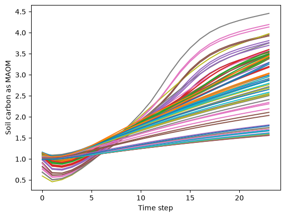
../_images/a45ba5b81c7284d43ac84054b992acd74d9c2c12e8ede41f385d7edcef50e67b.png

Vertical structure#

The Virtual Ecosystem creates a vertical dimension that is used to record canopy heights and soil depths across the grid.

# Extract the x and y location of the grid cell centres and layer heights
# for all observations at a given time step.
time_index = 0

x_3d = (
    continuous_data["x"]
    .broadcast_like(continuous_data["layer_heights"][time_index])
    .to_numpy()
    .flatten()
    + 45
)
y_3d = (
    continuous_data["y"]
    .broadcast_like(continuous_data["layer_heights"][time_index])
    .to_numpy()
    .flatten()
    + 45
)
z_3d = continuous_data["layer_heights"][time_index].to_numpy().flatten()

# Extract the air temperature for those points to colour the 3D data.
temp_vals = continuous_data["air_temperature"][time_index].to_numpy().flatten()

# Generate a 3 dimensional plot of layer heights showing temperature.

fig = plt.figure(figsize=(10, 8))
ax = fig.add_subplot(projection="3d")

cmap = plt.get_cmap("turbo")
paths = ax.scatter(x_3d, y_3d, z_3d, c=temp_vals, cmap=cmap)
fig.colorbar(
    paths,
    ax=ax,
    orientation="vertical",
    shrink=0.6,
    label="Air temperature (°C)",
    pad=0.1,
)

ax.set_xlabel("Easting (m)")
ax.set_ylabel("Northing (m)")
ax.set_zlabel("Layer height (m)")

ax.set_xticks(cell_bounds)
_ = ax.set_yticks(cell_bounds)

../_images/099df55565a65cbcb1048144e8c348bbb31d751f851dcdca2dea559faccf90ca.png