Running the Virtual Ecosystem in Static Mode

Why use Static Mode?

Imagine standing in a rainforest clearing at dawn. The sun rises, mist lifts, and the forest slowly comes to life.

Now imagine you could pause parts of this scene — hold the soil moisture constant, freeze the behaviour of animals, or keep the microclimate unchanged — while the rest of the ecosystem continues to move through time.

This is the essence of the Static Mode in the Virtual Ecosystem model.

In complex systems where everything interacts it can be hard to isolate what’s causing what. Static Mode helps untangle this web by letting you “freeze” components like plants or animals while others remain dynamic. At each model step, static components reset to their original state (e.g. eaten leaves magically reappear) — like a controlled reset — so any change comes only from the active, evolving parts.

This setup enables targeted experiments within the full model framework. For example, you can test how vegetation responds to changing temperatures without feedback from soil moisture changes, or explore animal behaviour in a fixed vegetation landscape.

By choosing which components evolve over time and which stay fixed, Static Mode helps reveal drivers of ecological change - helping us understand not just what happens, but why.

Note

The Virtual Ecosystem model can, in theory, be run with any combination of one or more components held static (except core). However, not all combinations are equally meaningful. It’s worth considering your experimental goals carefully and selecting static–dynamic configurations that best support the processes you want to isolate or understand.

Using the static mode

This example demonstrates how to configure and run the Virtual Ecosystem with selected components held static (for more technical details, see). Specifically, we focus on hydrology by keeping the microclimate, vegetation, animals, litter, and soils fixed. This isolates hydrological processes and so we can examine how individual model parameters and process representations influence model behaviour.

We run two experiments:

• HydroDefault: ‘hydrology-only’ simulation with default configuration

• HydroDry: ‘hydrology-only’ simulation with reduced initial soil moisture

In practice this means:

• Microclimate is fixed: e.g., temperature and relative humidity stay constant

• Plants are static: e.g. water uptake, transpiration, and interception do not vary

• Soil microbes, litter, and animals do not feedback into hydrology

• Only hydrology processes evolve over time in response to precipitation

Finally, we compare their outputs to the default setup (ve_example) where all components run dynamically.

Note

This guide focuses on how to technically configure and run static mode, not on interpreting the experimental results. This enables you to adapt the setup to suit your own analysis goals.

The code below to run the Virtual Ecosystem and plot results uses a mixture of the command line (e.g. bash on Linux or MacOS, powershell on Windows) and python code. For the code run at the command line, we currently only show the syntax for using bash. On Windows, you will need to change the paths (for example, to C:\Users\username\Temp\...).

1: Run ve_example as a baseline

Before setting up static experiments, make sure you can run the model successfully. If you haven’t yet installed and executed the example, follow the example instructions to familiarise yourself with the setup.

Install the example code - do make sure that you don’t have an old copy of this example code in your temporary directory before starting this exercise!

%%bash
# Install the example data directory from the Virtual Ecosystem package
ve_run --install-example /tmp/

Show code cell output

Hide code cell output

Example directory created at:
/tmp/ve_example

Run the example model with the provided full configuration.

%%bash
# Run the example
ve_run /tmp/ve_example/config/data_config.toml \
  /tmp/ve_example/config/abotic_config.toml \
  /tmp/ve_example/config/animal_config.toml \
  /tmp/ve_example/config/hydrology_config.toml \
  /tmp/ve_example/config/litter_config.toml \
  /tmp/ve_example/config/plant_config.toml \
  /tmp/ve_example/config/soil_config.toml \
  --outpath /tmp/ve_example/out/ \
  --logfile /tmp/ve_example/out/ve_example.log

Show code cell output

Hide code cell output

Starting Virtual Ecosystem simulation.
Logging to: /tmp/ve_example/out/ve_example.log
* Loading configuration

pyrealm/<unknown>:71: SyntaxWarning: invalid escape sequence '\s'

* Saved compiled configuration: /tmp/ve_example/out/ve_full_model_configuration.toml
* Built core model components
* Initial data loaded
* Models initialised: soil, hydrology, abiotic, animal, litter, plants
* Saved model initial state
* Starting simulation
100%|██████████| 24/24 [00:51<00:00,  2.16s/it]
* Simulation completed
* Merged time series data
* Saved final model state
Virtual Ecosystem run complete.

2: HydroDefault experiment

Configure static components

Once the baseline run is complete, you can set up the experiment with default ‘hydrology-only’ (no changes to parameters or input data):

• This is essential: Create a new output folder: /ve_example/HydroDefault_out/. The Virtual Ecosystem output files have fixed names and cannot be overwritten; if they already exist in your output directory, the model will crash.

• Navigate to the /ve_example/out/ folder.

• Copy the ve_full_model_configuration.toml file and rename it, for example to HydroDefault_config.toml.

• In the new file, set static = true for all components except hydrology and core, e.g.:

  [abiotic]
  static=true
  

Run HydroDefault experiment

Now run the model with the new configuration from your command line and make sure that the --outpath command in the second line is followed by the directory of the new output folder that you just created (here /tmp/ve_example/HydroDefault_out/), and the --logfile command in the third line is followed by the same path and a new file name ending in .log:

%%bash
ve_run /tmp/ve_example/static_config/HydroDefault_config.toml \
  --outpath /tmp/ve_example/HydroDefault_out/ \
  --logfile /tmp/ve_example/HydroDefault_out/HydroDefault.log

Show code cell output

Hide code cell output

Starting Virtual Ecosystem simulation.
Logging to: /tmp/ve_example/HydroDefault_out/HydroDefault.log
* Loading configuration

pyrealm/<unknown>:71: SyntaxWarning: invalid escape sequence '\s'

* Saved compiled configuration: /tmp/ve_example/HydroDefault_out/ve_full_model_configuration.toml
* Built core model components
* Initial data loaded
* Models initialised: soil, hydrology, abiotic, animal, litter, plants
* Saved model initial state
* Starting simulation
100%|██████████| 24/24 [00:05<00:00,  4.75it/s]
* Simulation completed
* Merged time series data
* Saved final model state
Virtual Ecosystem run complete.

Compare HydroConst results to baseline

To compare the results of the HydroDefault experiment to the fully dynamic ve_example, load the continuous results from /ve_example/out/ and /ve_example/HydroDefault_out/:

import matplotlib.pyplot as plt
import xarray

# Example: load or define your datasets
ve_example = xarray.load_dataset("/tmp/ve_example/out/all_continuous_data.nc")
hydrodefault = xarray.load_dataset(
    "/tmp/ve_example/HydroDefault_out/all_continuous_data.nc"
)

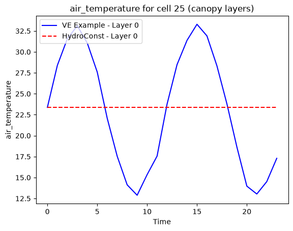
Air temperature above the canopy

The air temperature above the canopy is provided by an external data source at each time step. In the dynamic abiotic mode, this input is a time series to the Virtual Ecosystem that changes over time, allowing the model to respond to seasonal variation in atmospheric conditions. In static abiotic mode, by contrast, the same temperature value is used repeatedly for every time step throughout the simulation (think of groundhog day, the movie).

This difference has important implications for the hydrology model behaviour. In dynamic abiotic mode, fluctuations in air temperature can drive changes in evaporation, soil moisture, and other hydrological processes, leading to more realistic diurnal and seasonal cycles. In static abiotic mode, these processes may stabilize at an artificial equilibrium that reflects the constant atmospheric forcing rather than natural variability. This makes the static mode useful for isolating the role of internal model dynamics, but less representative of real-world conditions.

Show code cell source

Hide code cell source

# Choose the variable, cell_id to plot
var_name = "air_temperature"
cell_to_plot = 25

# Select the canopy layers
atmosphere_layers = ve_example.layers[0:1]

# Plot for each of the canopy layers
for layer in atmosphere_layers.values:
    plt.plot(
        ve_example["time_index"],
        ve_example[var_name].sel(cell_id=cell_to_plot, layers=layer),
        label=f"VE Example - Layer {layer}",
        linestyle="-",
        color="blue",
    )
    plt.plot(
        hydrodefault["time_index"],
        hydrodefault[var_name].sel(cell_id=cell_to_plot, layers=layer),
        label=f"HydroConst - Layer {layer}",
        linestyle="--",
        color="red",
    )

plt.xlabel("Time")
plt.ylabel(var_name)
plt.title(f"{var_name} for cell {cell_to_plot} (canopy layers)")
plt.legend()
plt.show()

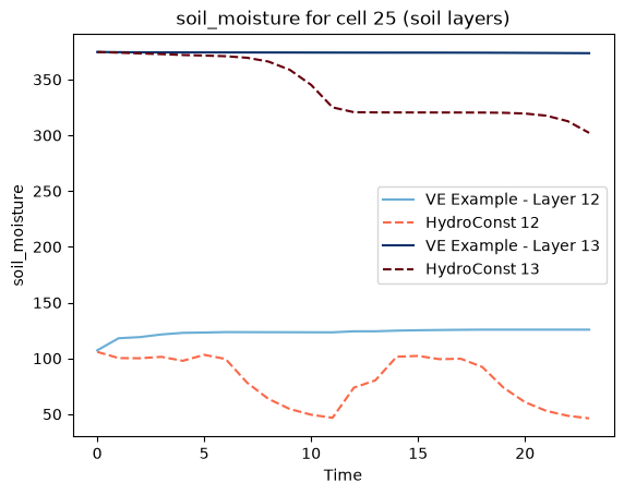
Soil moisture

The next figure shows the evolution of soil moisture over time. Interestingly, the results appear identical for both the ve_example and HydroDefault scenarios. This suggests that, under the conditions tested, soil moisture dynamics may be relatively insensitive to fluctuations in abiotic conditions — or that other model components dominate the response. However, understanding why this occurs would require a deeper investigation into the model’s energy and water balance under both configurations.

Show code cell source

Hide code cell source

import matplotlib.cm as cm
import numpy as np

# Choose the variable and cell_id to plot
var_name = "soil_moisture"
cell_to_plot = 25

# Select the bottom two layers (soil layers)
soil_layers = ve_example.layers[-2:]
n_layers = len(soil_layers)

# Choose colormaps for each dataset
ve_cmap = cm.Blues(np.linspace(0.5, 1, n_layers))  # Blue shades for ve_example
hydro_cmap = cm.Reds(np.linspace(0.5, 1, n_layers))  # Red shades for hydrodefault

# Plot for each of the bottom two layers
for i, layer in enumerate(soil_layers.values):
    plt.plot(
        ve_example["time_index"],
        ve_example[var_name].sel(cell_id=cell_to_plot, layers=layer),
        label=f"VE Example - Layer {layer}",
        linestyle="-",
        color=ve_cmap[i],
    )
    plt.plot(
        hydrodefault["time_index"],
        hydrodefault[var_name].sel(cell_id=cell_to_plot, layers=layer),
        label=f"HydroConst {layer}",
        linestyle="--",
        color=hydro_cmap[i],
    )

plt.xlabel("Time")
plt.ylabel(var_name)
plt.title(f"{var_name} for cell {cell_to_plot} (soil layers)")
plt.legend()
plt.show()

4: HydroDry experiment

Configure lower initial soil moisture

To set up a hydrology-only experiment with a change in initial soil moisture, follow these steps:

• This is essential: Create a new output folder for your experiment, for example /ve_example/HydroDry_out/.

• Navigate to the /ve_example/out/ folder.

• Copy the ve_full_model_configuration.toml file and rename to HydroDry_config.toml. We moved this file to a separate folder /ve_example/static_config/.

• Check the status flags are set to static = true, for all but the hydrology model.

• Make further changes to your configuration for your experiment. Here, we modify the initial soil moisture from the default value of 0.5 to 0.3 (line 2 below):

  [hydrology]
  initial_soil_moisture = 0.3
  initial_groundwater_saturation = 0.9
  static = false

Run HydroDry experiment

Now run the model with the new configuration from your command line. Again, make sure that the --outpath command in the second line is followed by the directory of the new output folder that you just created (here /tmp/ve_example/HydroDry_out/), and the --logfile command in the third line is followed by the same path and a new file name ending in .log:

%%bash
ve_run /tmp/ve_example/static_config/HydroDry_config.toml \
  --outpath /tmp/ve_example/HydroDry_out/ \
  --logfile /tmp/ve_example/HydroDry_out/HydroDry.log

Show code cell output

Hide code cell output

Starting Virtual Ecosystem simulation.
Logging to: /tmp/ve_example/HydroDry_out/HydroDry.log
* Loading configuration

pyrealm/<unknown>:71: SyntaxWarning: invalid escape sequence '\s'

* Saved compiled configuration: /tmp/ve_example/HydroDry_out/ve_full_model_configuration.toml
* Built core model components
* Initial data loaded
* Models initialised: soil, hydrology, abiotic, animal, litter, plants
* Saved model initial state
* Starting simulation
100%|██████████| 24/24 [00:05<00:00,  4.64it/s]
* Simulation completed
* Merged time series data
* Saved final model state
Virtual Ecosystem run complete.

Compare HydroConst and HydroDry results

To compare the results of different initial soil moisture levels in the hydrology-only configuration, load the continuous results from /ve_example/HydroDry_out/:

hydrodry = xarray.load_dataset("/tmp/ve_example/HydroDry_out/all_continuous_data.nc")

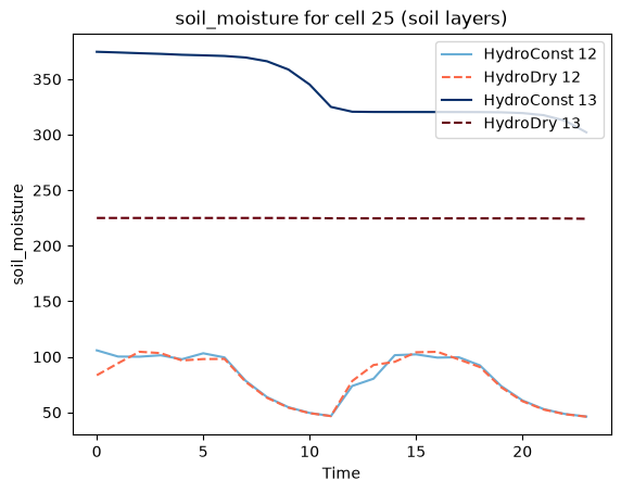
Soil moisture initial conditions

Now plot the soil moisture over time for both experiments. You will see that while the lower soil layer reaches a similar level in both runs after a few time steps, the top soil layer stabilizes at a different level. This suggests that initial conditions may influence the longer-term behaviour of some variables, even in a simplified setup.

One possible explanation is that the upper soil layer responds more directly to atmospheric conditions and surface fluxes, and may therefore retain some memory of its initial state. In contrast, the deeper soil layer could be less sensitive to short-term changes and more likely to converge across scenarios. However, this behaviour requires further investigation to understand the underlying dynamics, especially in the context of a static configuration.

Show code cell source

Hide code cell source

# Choose the variable and cell_id to plot
var_name = "soil_moisture"
cell_to_plot = 25

# Select the bottom two layers (soil layers)
soil_layers = ve_example.layers[-2:]
n_layers = len(soil_layers)

# Choose colormaps for each dataset
ve_cmap = cm.Blues(np.linspace(0.5, 1, n_layers))  # Blue shades for ve_example
hydro_cmap = cm.Reds(np.linspace(0.5, 1, n_layers))  # Red shades for hydrodefault

# Plot for each of the bottom two layers
for i, layer in enumerate(soil_layers.values):
    plt.plot(
        hydrodefault["time_index"],
        hydrodefault[var_name].sel(cell_id=cell_to_plot, layers=layer),
        label=f"HydroConst {layer}",
        linestyle="-",
        color=ve_cmap[i],
    )
    plt.plot(
        hydrodry["time_index"],
        hydrodry[var_name].sel(cell_id=cell_to_plot, layers=layer),
        label=f"HydroDry {layer}",
        linestyle="--",
        color=hydro_cmap[i],
    )

plt.xlabel("Time")
plt.ylabel(var_name)
plt.title(f"{var_name} for cell {cell_to_plot} (soil layers)")
plt.legend()
plt.show()